In the previous post, we dived deep into abstract algebra to motivate why Geometric Deep Learning is an interesting topic. Now we begin the journey to show that it is also useful in practice. In summary, we know that symmetries constrain our hypothesis class, making learning simpler—indeed, they can make learning a tractable problem. How does this happen?

Error sources in learning systems

For this to understand, we need to review the different error sources in learning systems, namely

• approximation: although neural networks have universal approximation capabilities, as in practice we cannot have infinitely deep and wide models, the function class the network can learn is constrained, i.e., it might not contain the ground-truth function;
• statistical: not just our model, but our samples are also finite; thus, training probably won’t find the true function. Our hope is that the statistical error gets smaller with smaller function class
• optimization: gradient descent is capable for a lot of things, but the (numerical) optimization procedure has many fallacies from local optima to numerical problems

Why should we use geometric priors?

Geometric priors in this context means exploiting the geometric structure of the data

For example, we can exploit that translating images will not change the object represented; thus, we get the same class label—some data augmentation techniques also rely on this idea, but they are not as principled as the Geometric Deep Learning approach. We will come back to this at the end of the post. This translation invariance is exactly what CNNs realize, leading to a simpler and smaller hypothesis class and thus smaller statistical error (and hopefully not increasing the approximation error—for CNNs, we know that labels are the same when images are translated, so we can be sure that the approximation error will not increase, but this can be nontrivial in more complex scenarios). Additionally, as CNNs do not care about translations, we don’t need to present images of the same object in every position; thus, we can reduce sample complexity too.

What are these geometric structures (domains)?

As the title of Geometric Deep Learning: Grids, Groups, Graphs, Geodesics, and Gauges says, deep learning is also invaded by the 5G: grids, groups, graphs, geodesics, and gauges (this has nothing to do with the conspiracy theories, probably because much fewer people understand it). The meaning of these concept will be clarified (not everything in this post). For now, what is important is that they describe (geometric) structure. Grids (e.g., pixel grids describing images) have an adjacency structure, i.e., all pixel has a specific set of neighbors. In the case of graphs, the edges between the nodes gives the structure. We would be fools not to exploit this structure. To refer to such structures, we will use the notion of

A domain $\Omega$ is a set with possibly additional structure.

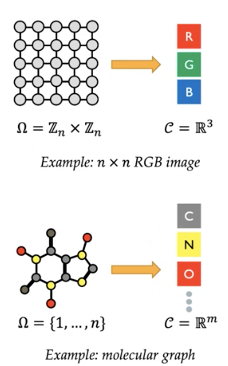
Sometimes, the domain itself is the data we use, for example

• point clouds (when the data consists only of the positions, but have not color or other attributes)
• meshes/graphs without node/edge features (when we have a social network of people, but we do not store their age, gender, or any related data—what a utopistic thought in today’s world, isn’t it?): in this case we can use the adjacency matrix

Nonetheless, often we want to store more information, e.g. the color of a pixel or what you have eaten for breakfast tomorrow with the obvious reason to sell it to marketers to create personalized ads for the special omelette with peanut butter and jelly you thought you can keep secret.

How can we represent further attributes (signals)?

For attaching other attributes to elements of a domain $\Omega$, we will apply a function, which we call the signal, mapping from elements of $\Omega$ (e.g., a pixel) to a vector space $C$ (e.g., RGB color of a pixel) and we denote the space of signals as $X={x:\Omega\to C}$ (think of this as the data space of RGB images).

So a signal associates a vector space $C$ for each element of $\Omega$.

$C$ does not even need to be the same for all $u$, it can be e.g. the tangent space of a specific point on a sphere.

What is interesting is that irrespective of the domain $\Omega$, $X$ will always be a vector space (linear combinations work as expected). Okay, it is not as interesting as we defined $C$ to be a vector space. Nonetheless, this enables us to do operations on our data (e.g., we can add images)—and as we know from our discussion on abstract algebra, operations are essential to define groups for example. Obviously, this is where today’s discussion will lead to.

What are symmetries?

We have done the above (and the previous post too) to be able to describe symmetries.

Symmetries are object transformations that leave the object unchanged,

and come in many flavors. Formulated otherwise: $g:\Omega\to\Omega$ is a symmetry if it preserves the structure of the domain. We start by noting that when using the group action $g$ we act on an element of $\Omega$ and get back a (possibly different) element of $\Omega$. This means that the mapping is $G\times\Omega \to \Omega$ and is denoted as $(g,u)\mapsto gu$ (i.e., it associates the element $gu$ to the element $u\in\Omega$ via the symmetry $g$).

$g$ has the following properties ($e$ is the identity element)

• Composition: $g(hu)=(gh)u$
• $eu=u$

Example

An example is planar motion in $R^2$, where $g$ is described by a rotation angle $\theta$, and two translation coordinates $t_x, t_y$. Then applying $g$ on a point $u=(x,y)$ can be characterized by the mapping $((\theta, t_x, t_y), (x,y))\mapsto [R; T] (x,y,1)$, where $[R;T]$ is a shorthand for the transformation matrix that rotates $u$ by $\theta$ and translates it by $(t_x,t_y)$—the third coordinate is needed to describe this affine transformation with a single matrix.

How can we describe all symmetries?

It needed a lot of effort, but now we can make sense of it to describe groups:

If we collect all symmetries (of a specific $\Omega$) together, we get a symmetry group $G$ with a group operation as the composition of group elements.

From the [previousus post](https://rpatrik96.github.io/posts/2022/06/dgl1-foundations/, we know that:

• the identity need to be in the group
• composition of group elements is also in the group (thus, a symmetry)
• inverse is also a symmetry In our case, the group elements are function (rotations for example), but generally they are just set elements.

How can we classify symmetry groups?

Symmetry groups can be discrete (rotating an equilateral triangle with multiples of $120^\circ$ or flipping its vertices) or continuous (rotations in $SO(3)$). They can be commutative/non-commutative (flipping the vertices of a triangle then rotating it has a different result than first rotating then flipping).

How can we apply symmetries on our data?

As these transformations (functions) $g$ act on $\Omega$ but our data lives in the signal space $X(\Omega, C)$, we need to introduce the corresponding mapping on $X$ as well. Namely, we need to be able to express symmetries not just on the pixel grid, but also in the RGB channels (the vector space $C$).

Example

Let’s look into an example of moving a bug (I am not supposing that you get a bug in your code and move it into someone else’s) in an image by translation $t=(t_x,t_y)$. When we translate the bug by 5 pixels to the right (this would mean $t_x=5, t_y=0$), then to get the pixel value of the translated image at position $u$, we need to look up the original pixel value at the position 5 pixels to the left of $u$, i.e., at $u-t$.

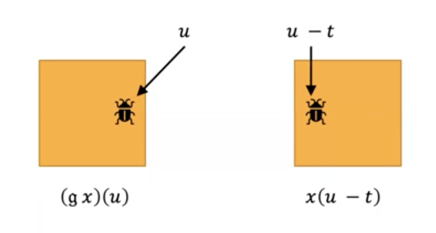
Symmetries in data space formula

This example highlights why the corresponding formula to define the symmetries of $\Omega$ acting on the signal space $X(\Omega, C)$ is \((gx)(u) = x(g^{-1}u)\), in our example $g^{-1}$ is applying $-t$. If you wonder what is the reason for the inverse, you don’t need to wait further: it is to satisfy the group axioms (hint: inverse element needs to be in the group—in our example, this is the relationship between the shifted pixels to the left/right).

Groups get into action: how do we get to representations?

Groups are abstract concepts, we need to describe them such that our computers can produce significant carbon footprints. Implicitly, we already did this (not the carbon footprint thing though): when we used matrices to describe affine transformations, we assigned a linear map to the group element of $(\theta, t_x, t_y$). Basically, this is what representations do.

An $n$-dimensional real representation of a group $G$ is a map $\rho: G\to R^{n\times n}$ assigning an invertible matrix $\rho(g)$ to each $g\in G$ such that it satisfies the homomorphism property \(\rho(gh) = \rho(g)\rho(h)\)

Example

An example would be the following:

• group $G=(Z,+)$
• domain $\Omega = Z_5 = {0,1,2,3,4}$ (a short audio signal of length five)
• action of $g=n$ on $u\in\Omega: (n,u)\mapsto n+u$ (mod 5)
• the representation of $X(\Omega)$ is a 5-dimensional shift matrix

An important conclusion is that the number of elements in $G$ (in this case infinite) and the dimension of the representation are independent

What are the types of symmetries relevant to machine learning?

Symmetries of parametrization

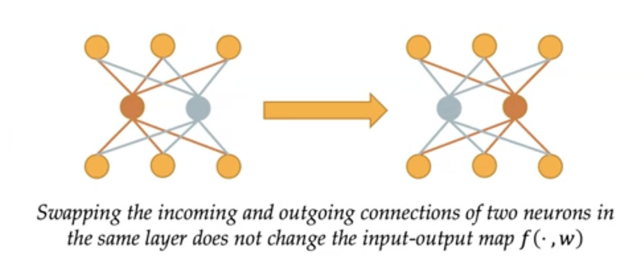
This type of symmetry comes from how we build our neural networks. For example, given the vector space of data (signals) $X$, outputs (e.g., labels) $Y$, and the weights $W$, we can describe our net by a mapping $X\times W\to Y$ (mapping data with the net’s weights to a label) and say that a transform $g$ is a symmetry of this parametrization (~network structure) when we get the same result by using the weights $w\in W$ as with $gw$. For example, in an MLP permuting the hidden units makes no change in the output as we add the values and addition is commutative.

Symmetries of the label function

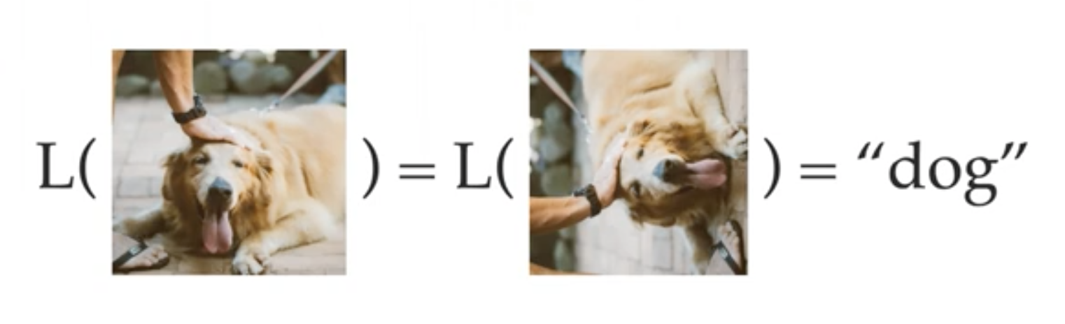
We already touched on CNNs and their invariance w.r.t. translation. In general, if the label does not change under a transformation $g: \Omega\to\Omega$, then we say that $g$ is a symmetry of the label function. The label function is simply a notation describing the mapping that associates a label in $Y$ to a data point in $X$ (denoted by $L: X\to Y$ ). Note that here $g$ is applied on the domain, only after that comes the label function, i.e., $L\circ g $.

This means that if we have a single data point but know all $g\in G$, then we can generate all instances of the class. Basically, learning all symmetries is what it takes to solve classification (which is a very hard problem).

From the previous post, we can relate to factor groups, which describe the subgroups of a specific group that behave the same way w.r.t. the kernel of an operation. What this means for classification is that the elements of factor groups divide all samples into the respective classes. So we can think of the symmetries of the label function as a way to describe the elements of the factor group.

Why should we really use geometric priors?

Because they have symmetries! And now we can describe them. For example:

• For sets, permuting the elements does not change the set (i.e., the structure of the domain).
• Grids (as we have seen with the image example before) have symmetries w.r.t. discrete rotations, translations, etc
• Isometries (distance-preserving maps) leave the Euclidean space unchanged
• Diffeormorphisms preserve the smooth structure on $\Omega$

With such structures as graphs or sets, we can point out a seemingly subtle but important detail: although a graph (or a set) is an abstract concept, they need to have a practical description (how they are stored in computer memory). The consequence is that usually, we are interested in the symmetries of the description, not that of the object.

How can we exploit symmetries?

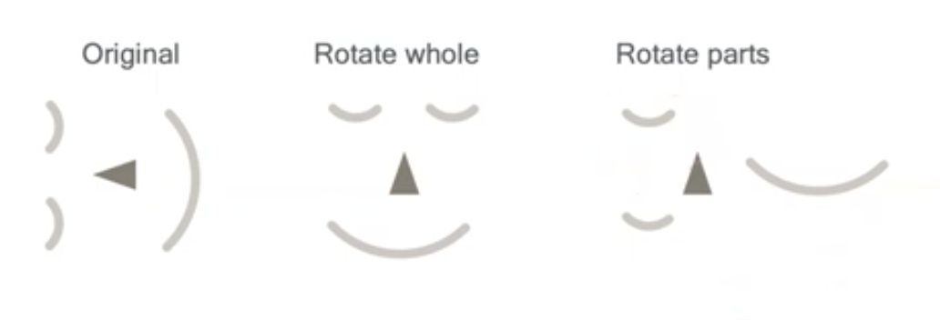
We already talked about CNNs and that they are invariant to translation. Nonetheless, invariance has its fallacies. In the case of learning faces, we need to be careful not to make the intermediate representations invariant, for that can lead to unrealistic objects, e.g., with faces this would mean the right most image below.

What is the answer to that? Equivariance

Equivariant networks

Equivariance means that when transforming the input of $f$ with transform $h$ is the same as the output is transformed with the same $h$. \(f \circ h(u) = h\circ f(u)\)

We can build equivariant neural networks, if we have the follwoing components:

• feature vector spaces $X_i$
• nonlinear maps $f_i$
• symmetry group $G$
• group representations $\rho_i$ for each $X_i$

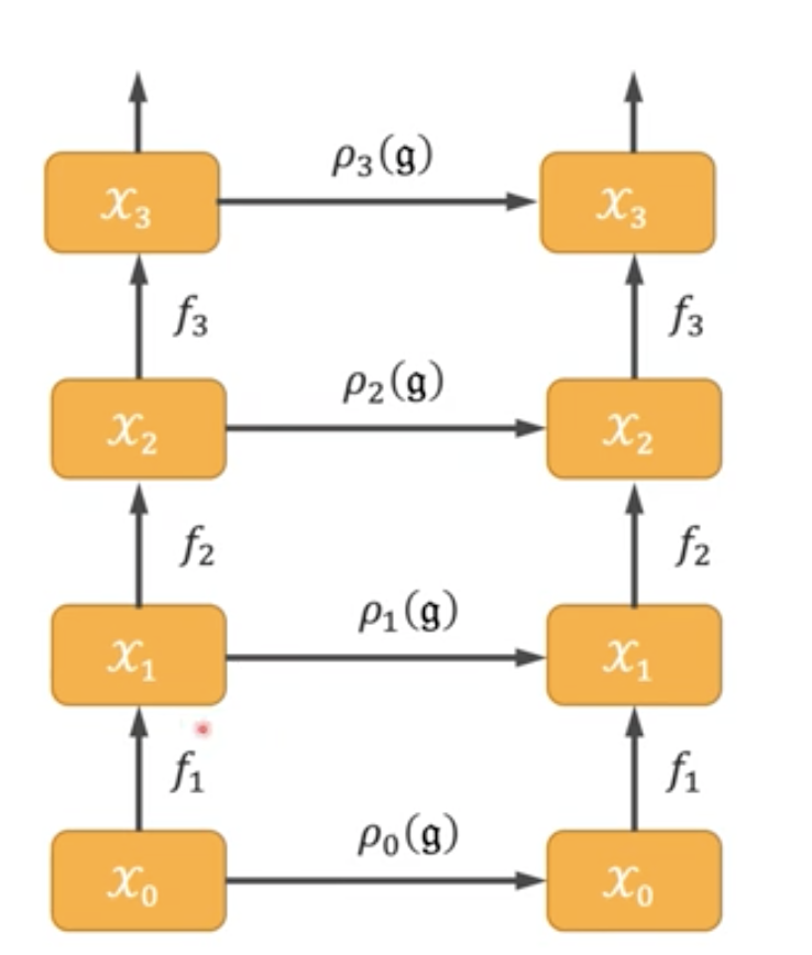
We need different group representations for each $X_i$ as the same symmetry “needs to be adapted” to the new data space $X_i$.

This leads to the definition of equivariant networks:

\(f_i \circ \rho_{i-1}(g) = \rho_i(g) \circ f_i,\) which means that applying the (corresponding) representation and the nonlinear map can be almost interchanged (note the different indices for $\rho$). First applying the representation of layer $i-1$ and then mapping through layer $i$ should give the same result as first mapping through layer $i$ then applying $\rho_i$.

Example

When treating images, $X_1$ is $n\times n \times 3$ (RGB channels), and assume that the first layer $f_1$ is a convolution with 64 channels. This means that we need a different representation of, e.g., translations in this 64-dimensional space (if we translate with $\rho_0$ then map with the first layer, we should get the same as if we would first map then translate with $\rho_1$). The rationale is that it cannot be that a translation can be described in the exact same way in both 3 and 64 dimensions.

Why is equivariance beneficial for generalization?

In the end, our goal is to generalize better: we want that all samples that map to the same feature will still map to the same feature after undergoing a transformation by the group representation $\rho_1(g)$ in the input space. For this, the notion of an orbit is a useful concept:

Orbit: the manifold of a sample undergoing a transformation by each element of a group (e.g. the manifold of all rotated digits, starting from a single one—these are the curved lines in the input space in the figure below).

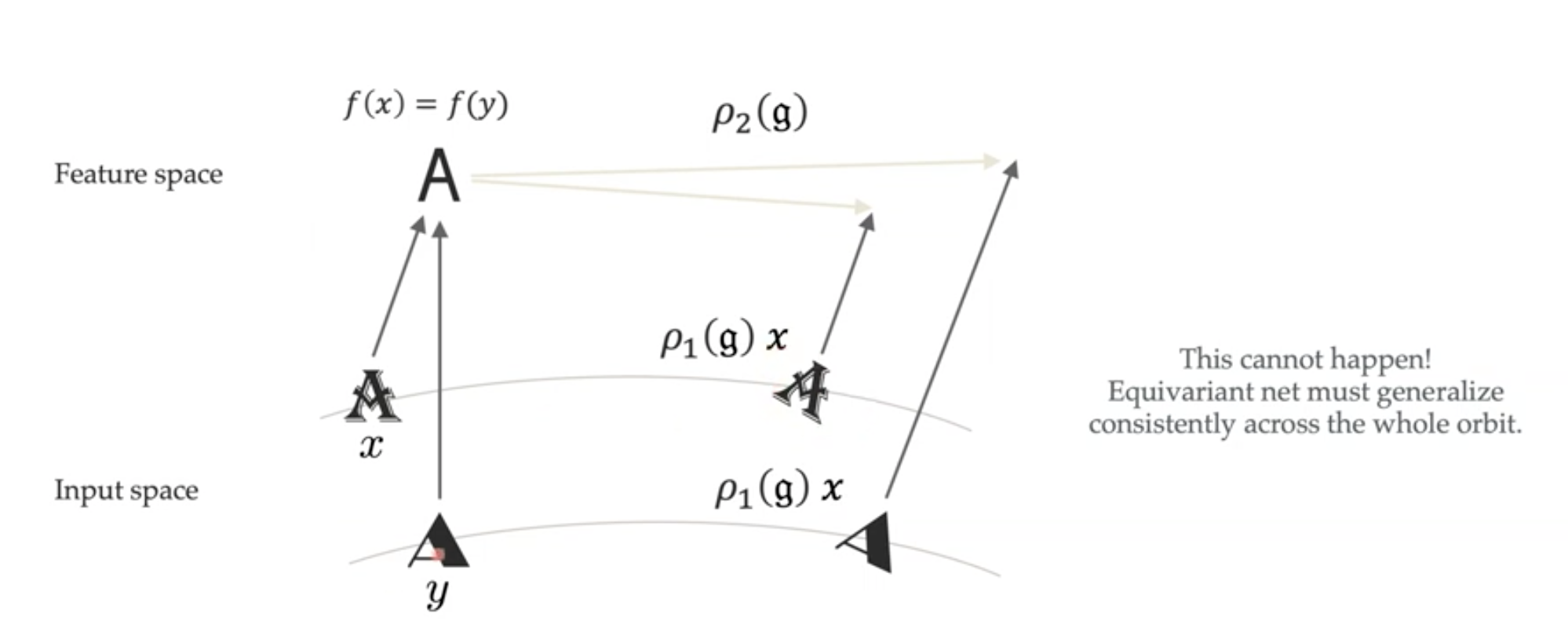
Indeed, this is what equivariant nets are capable of (see, e.g., this paper on CNNs).

Wait a second! We were talking about transformed samples, can’t we achieve the same generalization properties with data augmentation (instead of the toil required to derive the theory and design for equivariant models)?

No, data augmentation is inferior to equivariant networks.

For example, data-augmentation implements a constraint for the whole network (i.e., when augmenting the samples, we do not prescribe constraints for specific layers), but equivariance imposes a layer-wise constraint. And it scales better to large groups.

Summary

We dived deep into geometric priors to describe symmetries in the domain (data), parametrization, and labels with the goal to design efficient models exploiting this inductive bias. In the end, we did exactly that with equivariant networks and understand why equivariance is beneficial (principled way to generalization).

Acknowledgement

This post was created from the AMMI Course on Geometric Deep Learning - Lecture 3 held by Taco Cohen. Mistakes are my own.